75 slides extracted.
Slide 1 — 0:04 (watch)
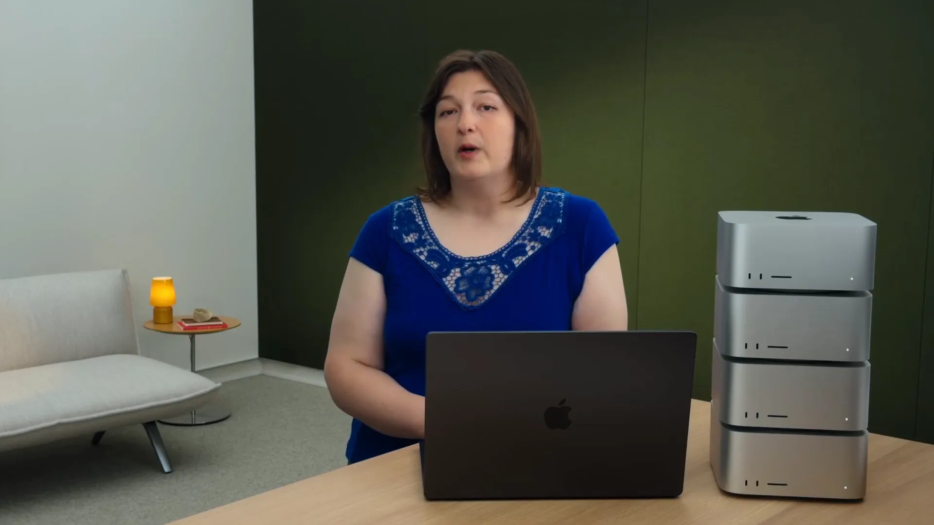
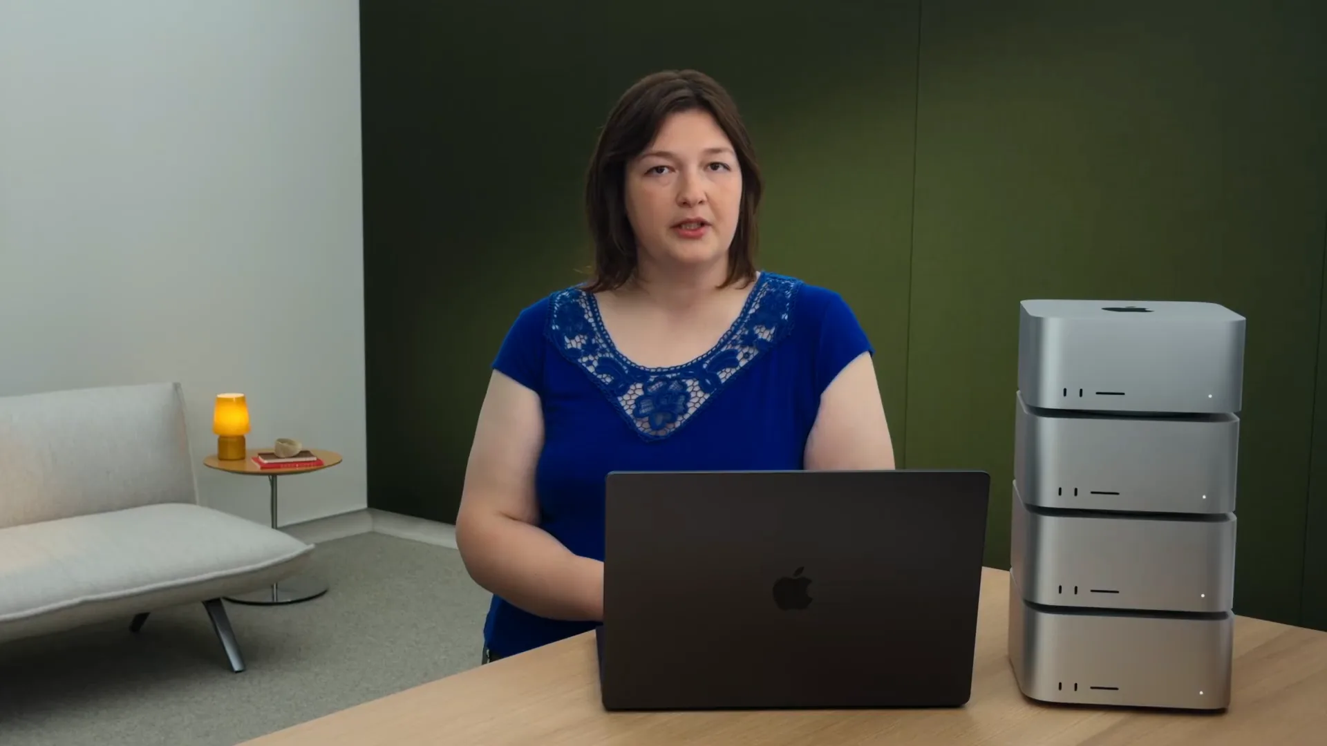
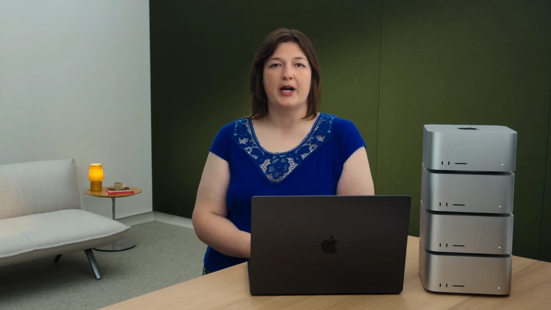
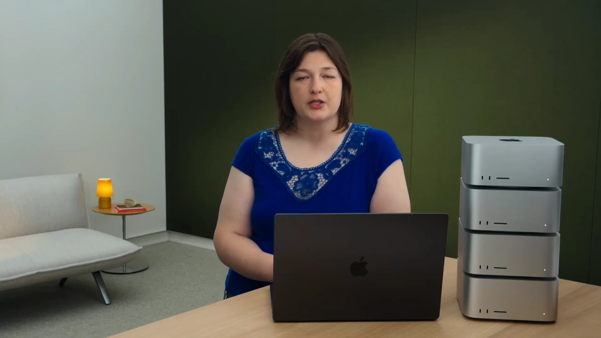
 | Hello, I'm Tatiana, a Research Scientist on the MLX team. |
Slide 2 — 0:20 (watch)
 | It's been a remarkable time for local LLMs. Models are continually increasing in size and gaining impressive capabilities, becoming smarter and tackling more challenging problems. As they improve, we leverage them for longer contexts, more complex tasks, and intricate workflows. Eventually, limitations arise in memory, compute, or bandwidth on a single machine. |
Slide 3 — 0:38 (watch)
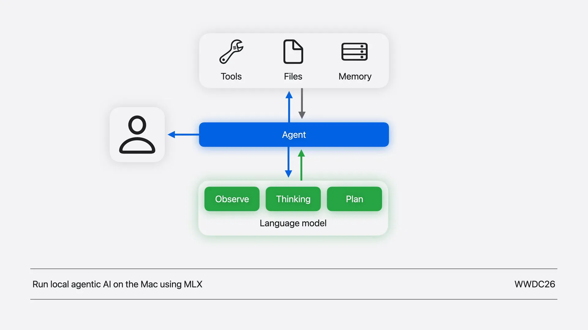
 | In our video, "Run Local Agentic AI on the Mac using MLX," we demonstrate how to run AI agents locally. |
Slide 4 — 0:52 (watch)
 | With multiple devices, you can enhance local AI by running larger LLMs or accelerating them through distributed inference and training. Today, we will explore scaling across multiple Macs with MLX using the hardware available on your desk. |
Slide 5 — 1:08 (watch)
 | We will begin with the command line interface to run models on your machines, then move to the Python API for experimentation, and conclude with Swift for embedding these workflows directly into your apps. Let's get started. |
Slide 6 — 1:20 (watch)
 | First, we will examine the complete hardware and software stacks that enable distributed workloads on Apple Silicon. |
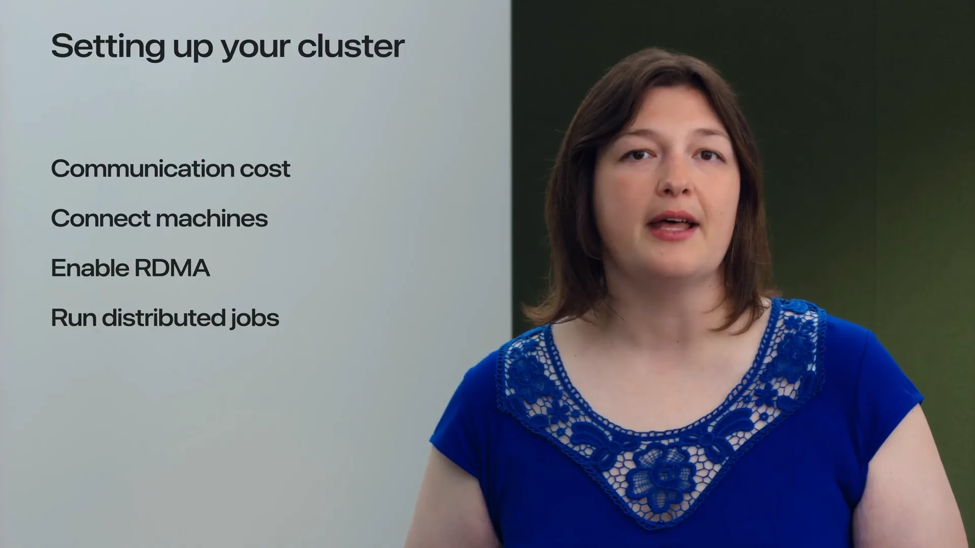
Slide 7 — 1:30 (watch)
 | Next, we will combine everything by turning four M3 Ultras into a cluster. We will walk through each step, selecting the appropriate topology to connect the machines, enabling fast communication, and launching distributed jobs. |
Slide 8 — 1:46 (watch)
 | Once the cluster is ready, we will focus on fast and local distributed LLM inference and fine-tuning. We will run it with MLX, compare it side by side against a single Mac, and examine how MLX distributes the model across the cluster. |
Slide 9 — 2:02 (watch)
 | Most examples will be presented in the command line interface. In the end, we will demonstrate how distributed communication is also accessible through Python, Swift, and C++ APIs. |
Slide 10 — 2:12 (watch)
 | Let's begin by examining distributed communication for Apple Silicon. |
Slide 11 — 2:16 (watch)
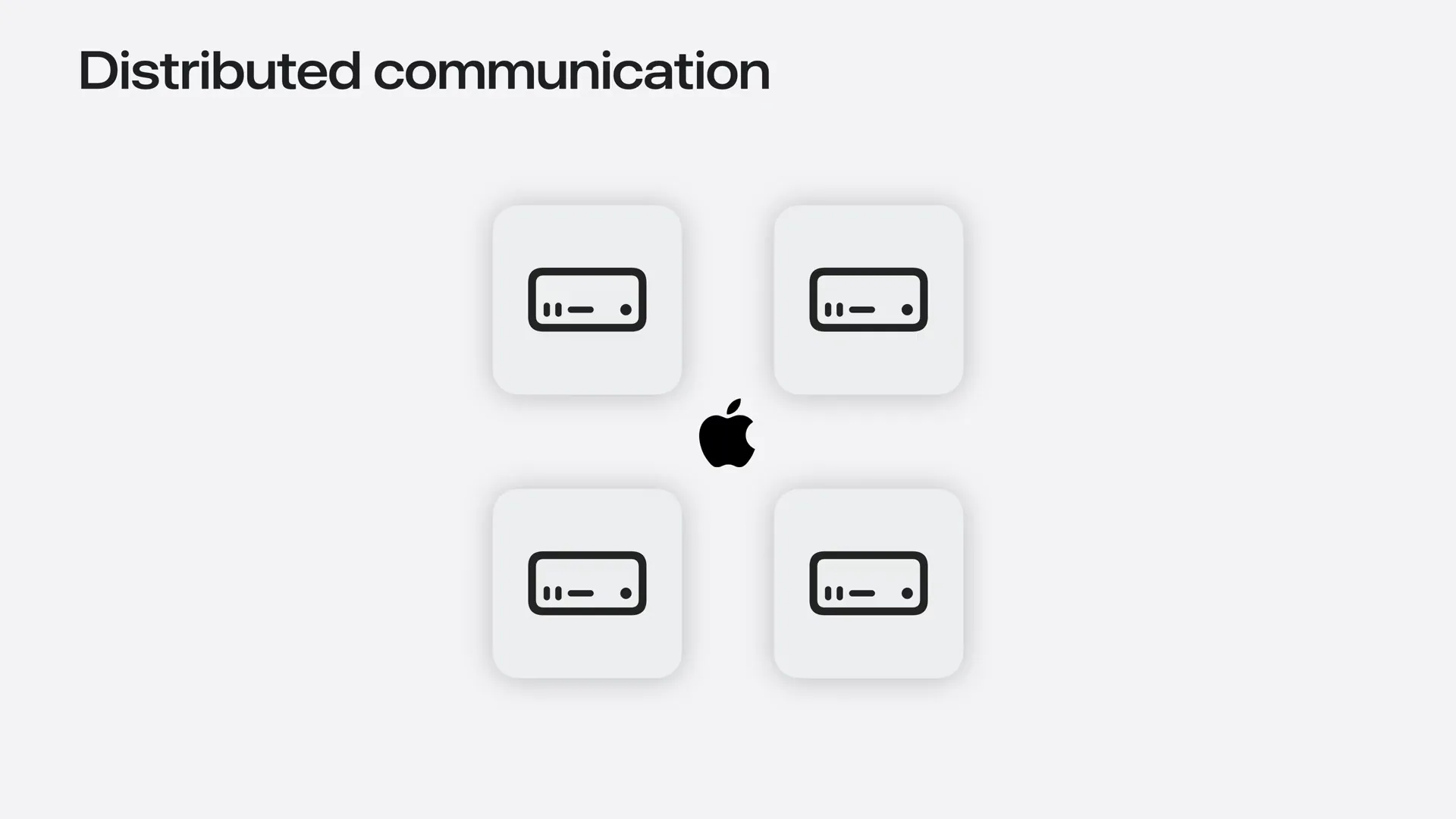 | To send and receive data quickly, machines must be connected through a physical link and interconnect. |
Slide 12 — 2:32 (watch)
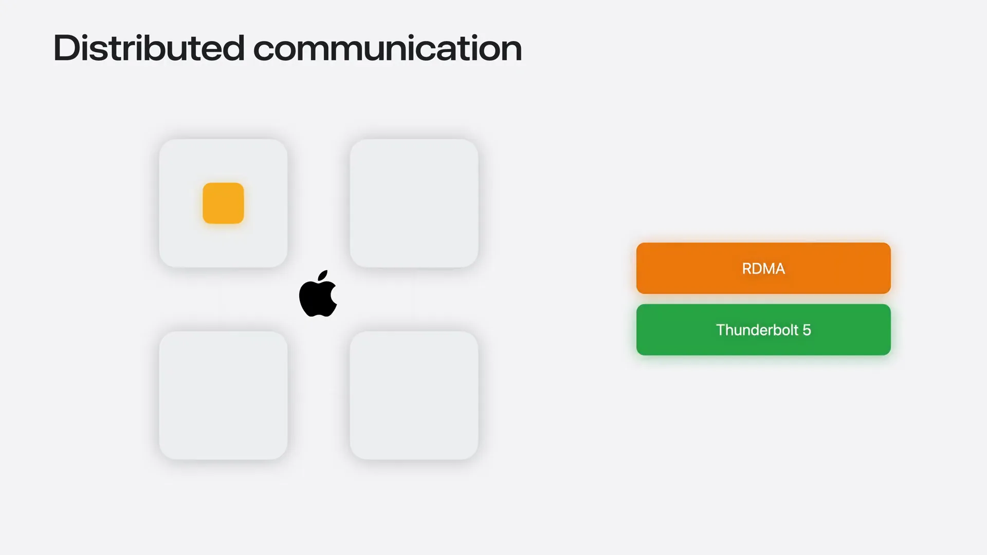 | We also need a transport protocol, which is a mechanism that transfers bytes from one machine's memory to another's. Starting in macOS 26.2, Remote Direct Memory Access Protocol, or RDMA, is supported over Thunderbolt 5. RDMA enables data to move directly from one machine's memory to another's, minimizing CPU and operating system overhead. |
Slide 13 — 2:56 (watch)
 | RDMA over Thunderbolt provides the high bandwidth and low latency communication necessary for distributed workloads. However, it only facilitates raw data movement between two machines. |
Slide 14 — 3:12 (watch)
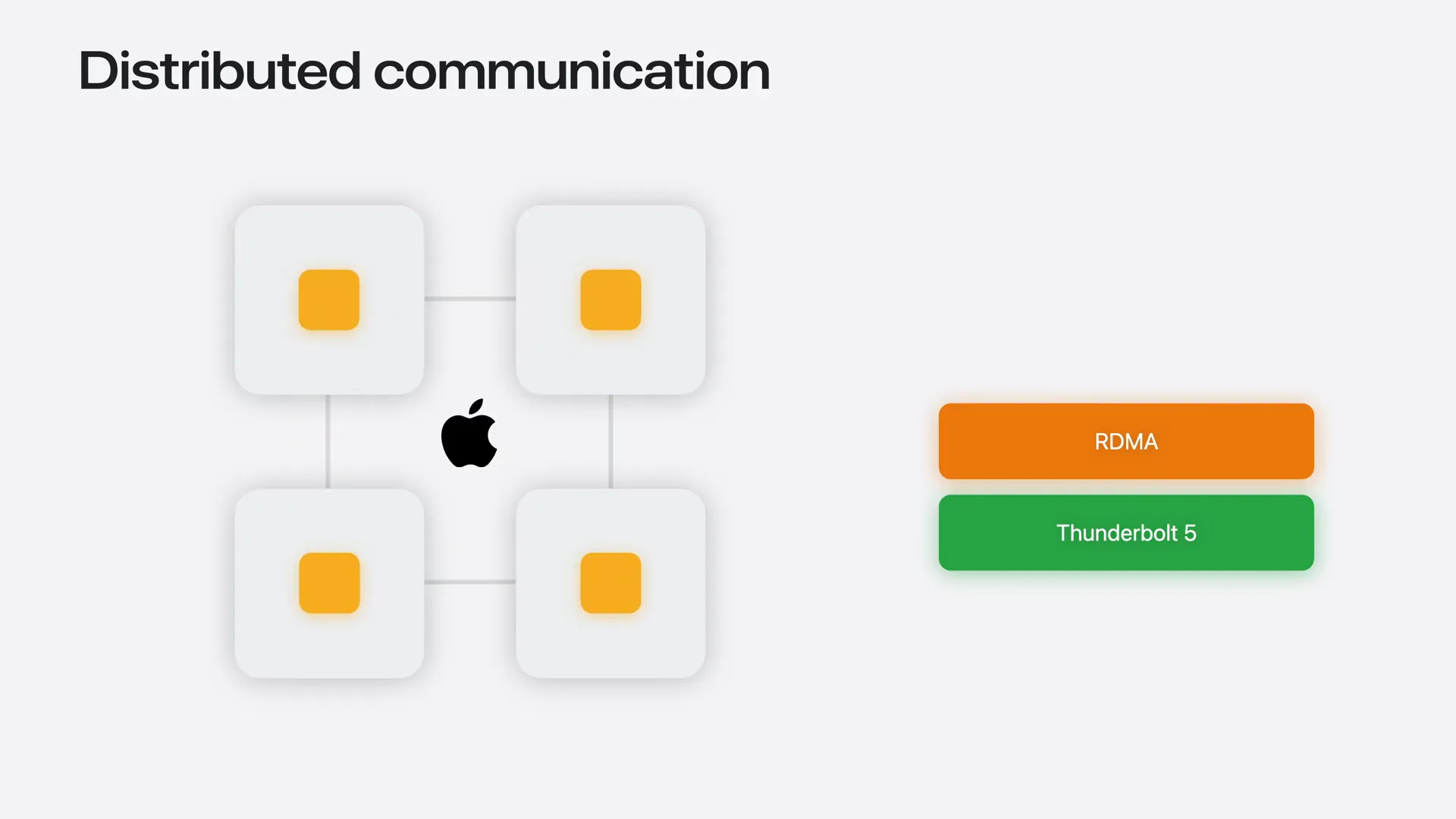 | Distributed programs require a higher-level communication backend that provides communication primitives for sending data between individual machines and coordinating across the entire group. These operations are essential building blocks for distributed training and inference. This is where Jackal comes in. |
Slide 15 — 3:34 (watch)
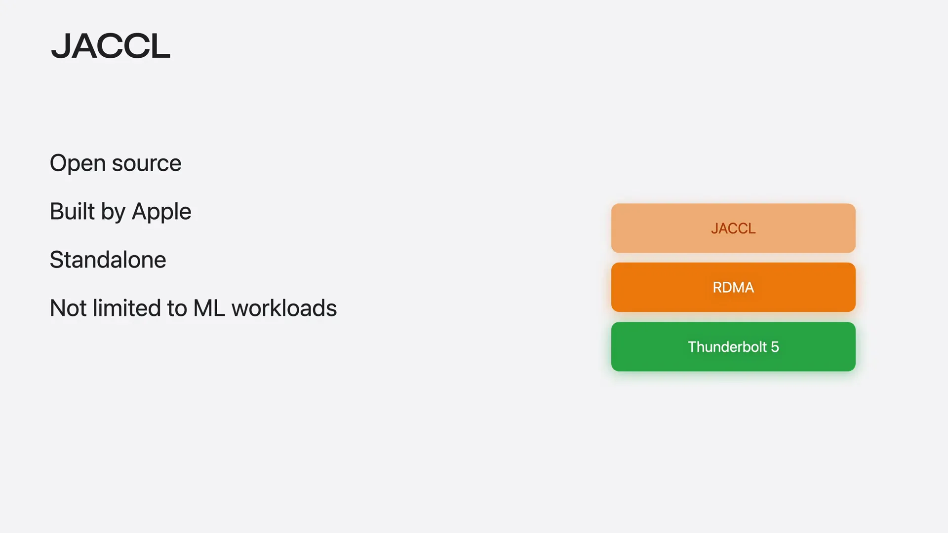 | Jackal is an open-source collective communication library developed by Apple. It leverages RDMA over Thunderbolt and provides collective communication primitives for sending data between machines and combining results across the group, all without requiring you to manage the low-level transport. Additionally, it is not limited to machine learning; any distributed workload on Apple Silicon can utilize it. |
Slide 16 — 3:52 (watch)
 | The final piece of the stack is a machine learning framework that utilizes the communication backend for distributed inference and training: MLX. |
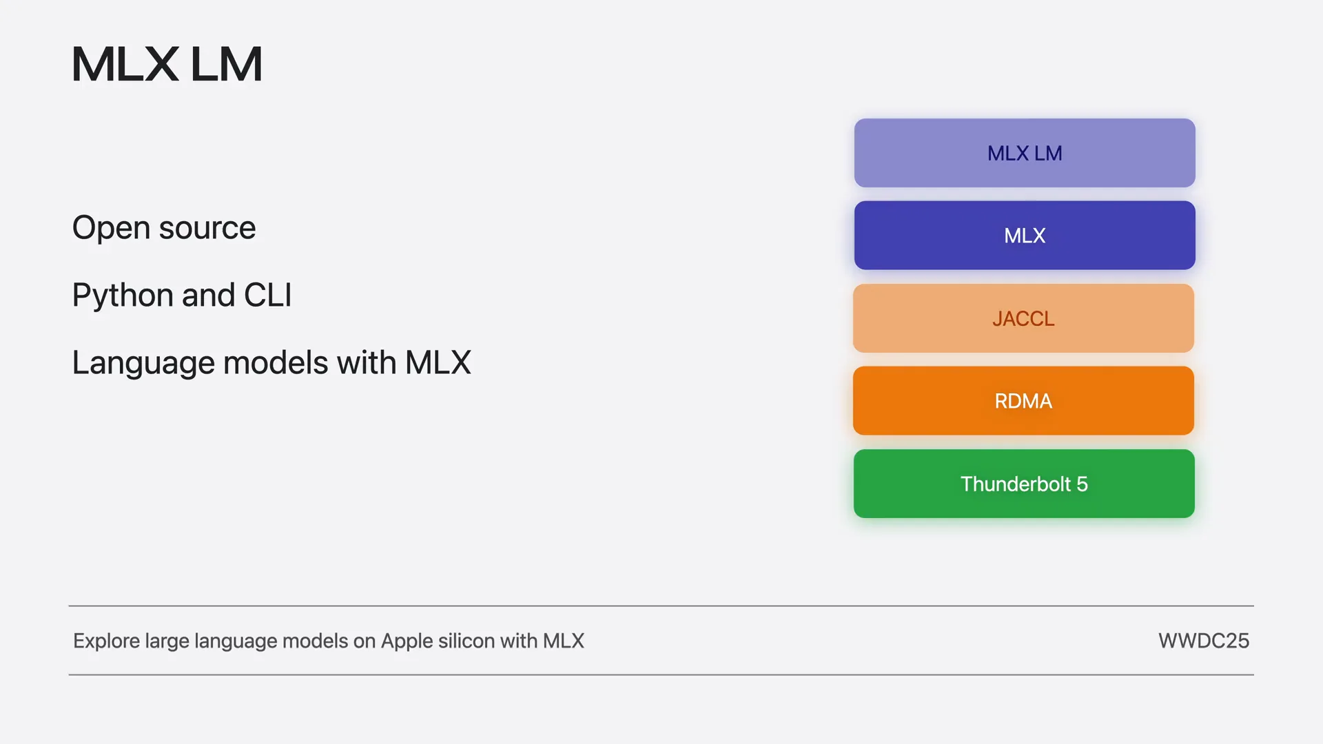
Slide 17 — 4:10 (watch)
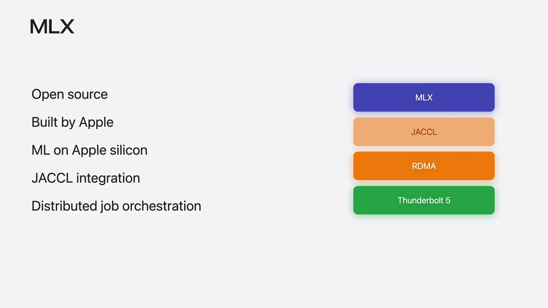 | MLX is an open-source machine learning library developed by Apple for Apple Silicon. It utilizes Jackal for low-latency distributed communication and offers tools for orchestrating distributed jobs across the cluster. If you are new to MLX, we recommend watching our video "Getting Started with MLX on Apple Silicon" from WWDC25. |
Slide 18 — 4:26 (watch)
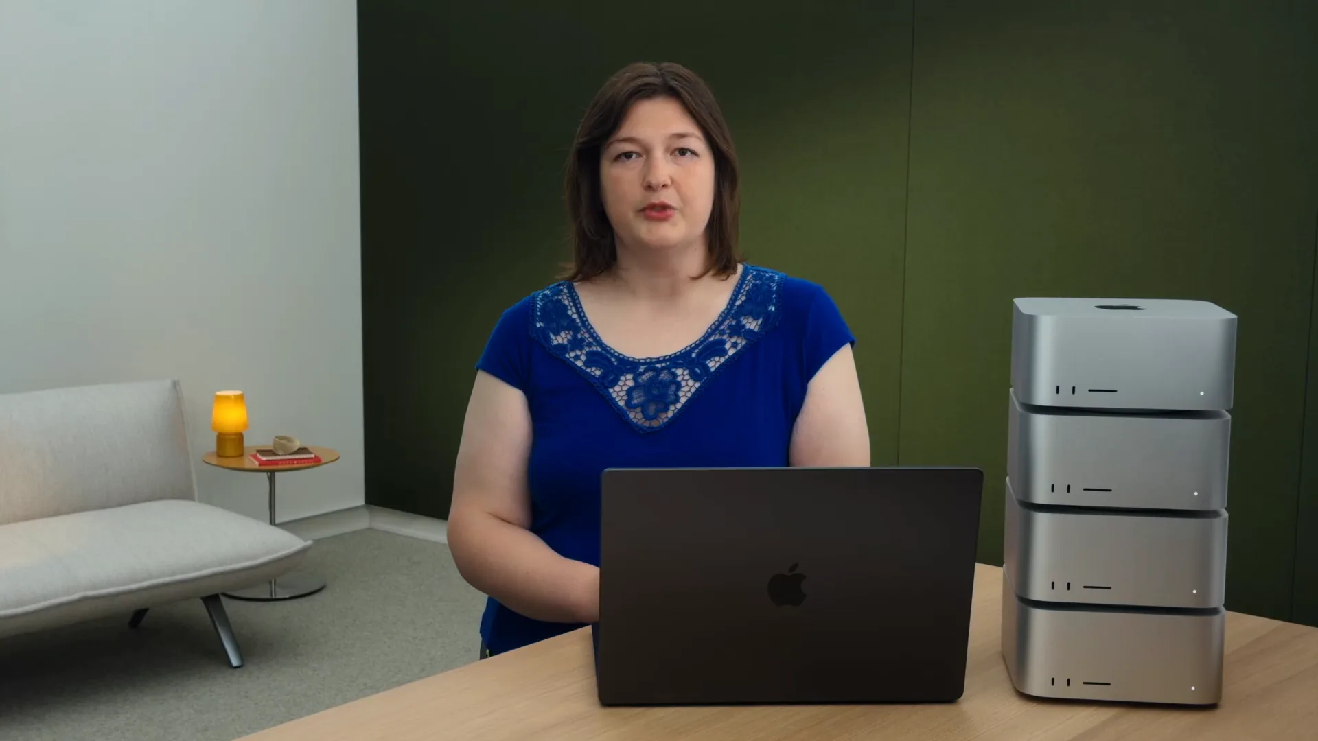
 | Now that we understand the full stack, let's put it all together and build a cluster, which is a group of machines working together on the same task. We will use four M3 Ultras. |
Slide 19 — 4:40 (watch)
 | To set up the cluster, we need to connect the machines using Thunderbolt 5 cables. There are various ways to wire them together, and the topology directly affects communication time. First, let's examine the factors that define that time. |
Slide 20 — 4:52 (watch)
 | Next, we will examine how to connect the machines, the topologies supported by Jackal, and the trade-offs associated with each topology. |
Slide 21 — 5:00 (watch)
 | Next, we will demonstrate how to enable RDMA on the machines for fast communication. Finally, we will launch distributed jobs on the cluster using MLX. |
Slide 22 — 5:28 (watch)
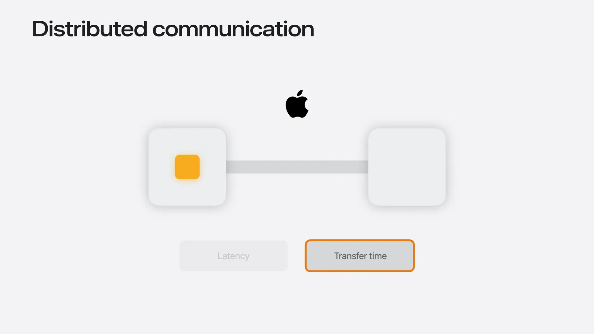 | Communication time consists of two components: latency and transfer time. Latency is the fixed cost incurred for each communication operation, regardless of the data size. Transfer time refers to the cost of moving data through the link, which increases with message size and is influenced by the link's bandwidth. For small messages, the cost of data movement is minimal, making latency the dominant factor. Conversely, for large messages, the situation reverses. Depending on whether communication is latency-bound or bandwidth-bound, different topologies may be preferred. |
Slide 23 — 6:18 (watch)
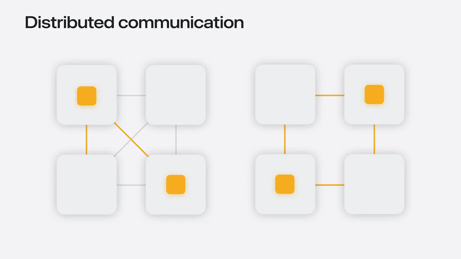 | Jackal supports two topologies: a mesh and a ring. In a full mesh, every machine connects directly to every other machine, resulting in the lowest possible latency for group communication. In a ring topology, each node connects only to its two neighbors, requiring communication between non-adjacent nodes to travel through intermediate machines, which increases latency. However, the ring topology requires fewer cables and ports per machine, making it easier to scale to more nodes. Each node has only two connections, allowing the use of extra Thunderbolt ports to run two or three cables per neighbor, depending on the MAC, which increases the bandwidth per link and reduces transfer time. When machines are connected in a mesh, we can route each communication through either the mesh or the ring topology. |
Slide 24 — 6:56 (watch)
 | Jackal automatically selects the optimal topology based on the message size and communication operation: it uses a mesh topology when latency is a priority and a ring topology when bandwidth is more critical. To take advantage of this flexibility, we will connect all M3 Ultras in a mesh configuration. |
Slide 25 — 7:08 (watch)
 | Now that we have connected all M3 Ultras together, we need to enable RDMA on all machines. |
Slide 26 — 7:20 (watch)
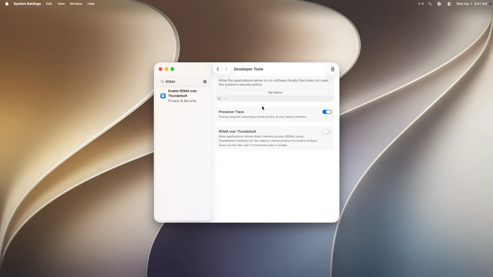 | Open Settings on each machine, search for RDMA, click on "Enable RDMA over Thunderbolt," enable RDMA, and then reboot the machine. |
Slide 27 — 7:32 (watch)
 | Great, Macs are connected with Thunderbolt 5 cables, and RDMA is enabled. Now we need a method to launch distributed programs. |
Slide 28 — 7:40 (watch)
 | One way to launch distributed programs is over the local network, using Wi-Fi or Ethernet. |
Slide 29 — 7:48 (watch)
 | From any machine with SSH access to the cluster, such as a MacBook in my case, we connect to each Mac, start the program, and from that point on, all machines communicate directly over the Thunderbolt links. |
Slide 30 — 8:02 (watch)
 | MLX provides a launch helper that automates this process for you. |
Slide 31 — 8:08 (watch)
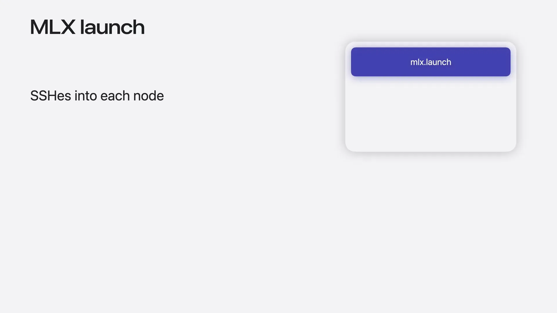 | You run MLX launch on your MacBook, and it orchestrates the cluster for you. |
Slide 32 — 8:12 (watch)
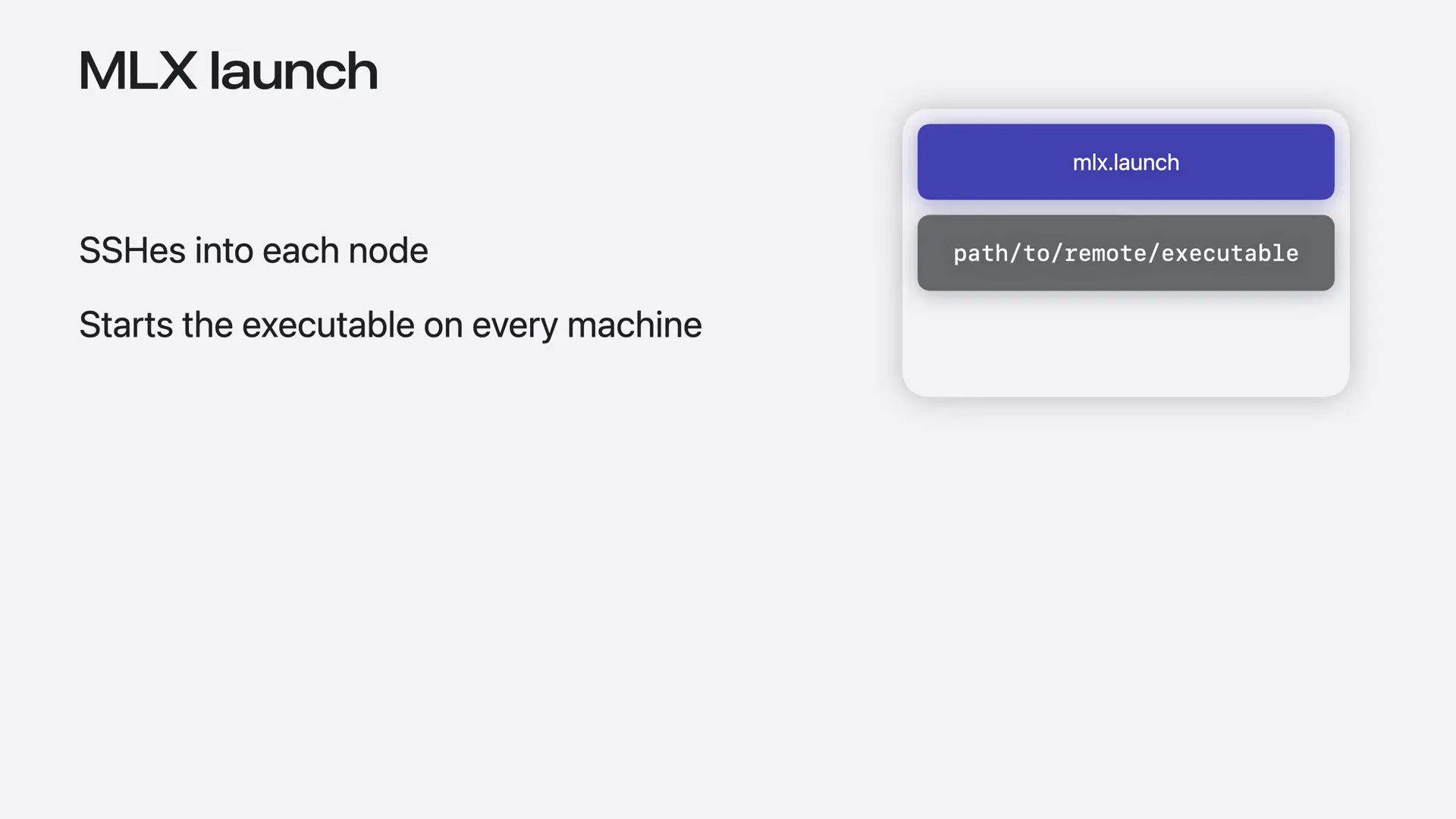 | You provide the executable you want to run and a JSON host file that describes your cluster. |
Slide 33 — 8:18 (watch)
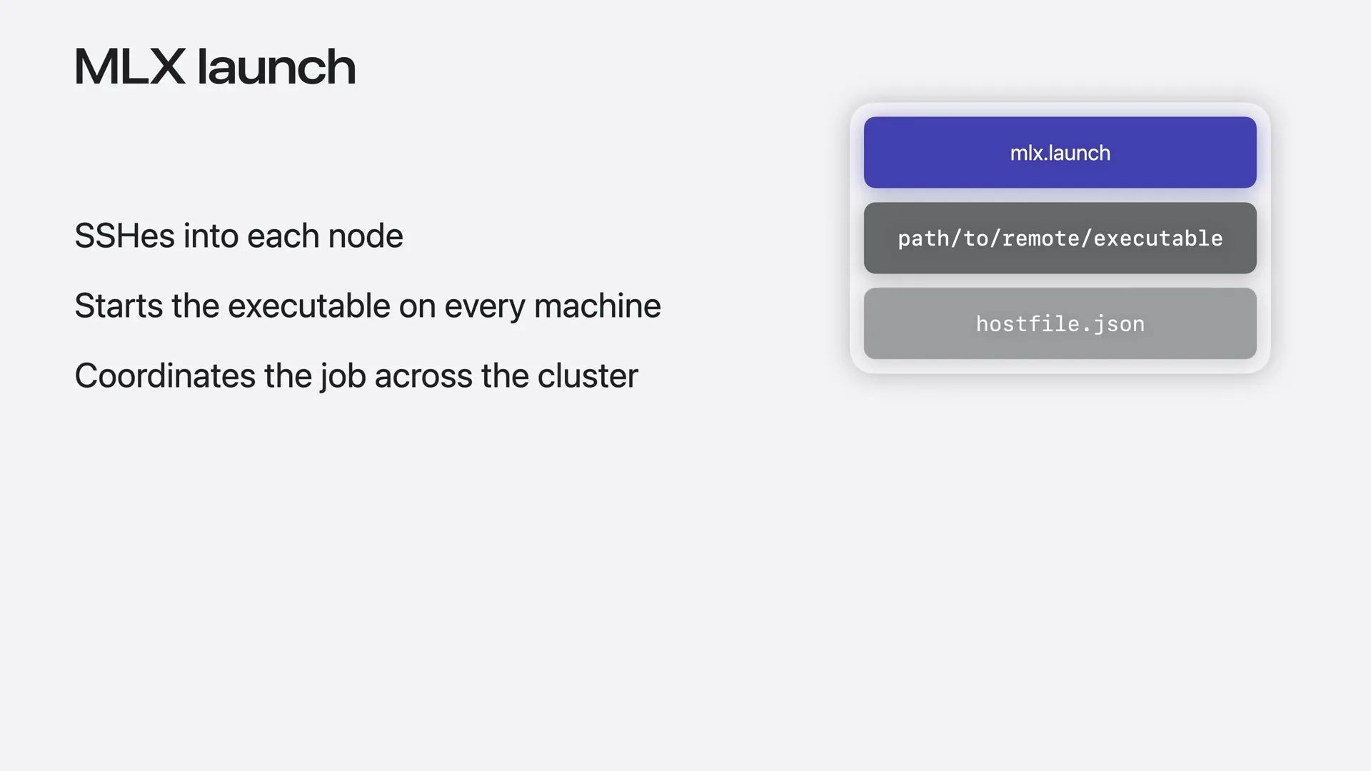 | From there, it SSHs into each node using the host names from the provided host file and starts the executable on every machine. |
Slide 34 — 8:28 (watch)
 | The host file that describes the cluster is structured as a JSON array, with one entry for each node. |
Slide 35 — 8:42 (watch)
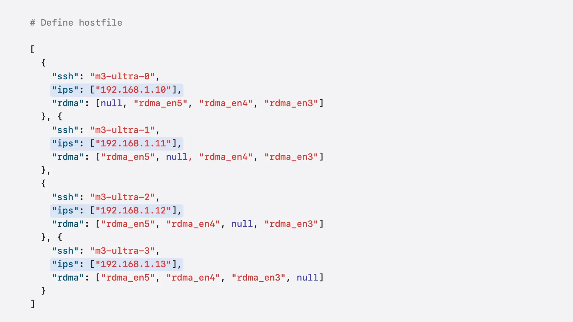 | The host file is a JSON array with one entry per node. The "SSH" field specifies the hostname used by MLX launch to connect to the machine. The "IPs" field contains the machine's IP address on your local network, which Jackal uses for initial coordination between nodes. The "RDMA" field lists the RDMA device names for each Thunderbolt peer connection. |
Slide 36 — 8:58 (watch)
 | You can write the configuration manually, but MLX also provides a helper script, MLX distributed config, that generates it for you. |
Slide 37 — 9:26 (watch)
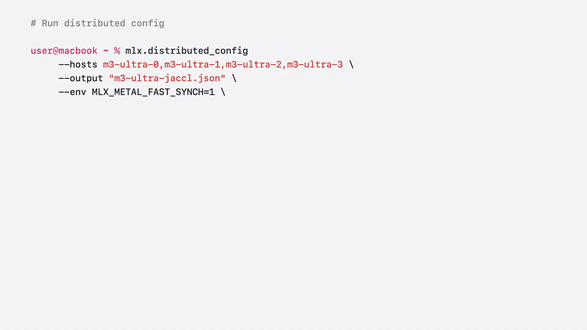 | You pass a list of host names and an output path, and you can embed environment variables in the config, which will be set automatically on every node at launch time. Here, we set MLX Metal Fast Sync to 1, enabling faster GPU-to-CPU synchronization. This is critical for distributed tasks because computation runs on the GPU while communication runs on the CPU. You can also pass the autosetup flag to configure the Thunderbolt network automatically. The communication backend argument defines whether the setup is a mesh or a ring. For a mesh, the backend is set to Jackal, as shown in this example. For a ring, you would change it to Jackal ring. |
Slide 38 — 9:50 (watch)
 | Let's run this command to generate the host file for our cluster. |
Slide 39 — 10:02 (watch)
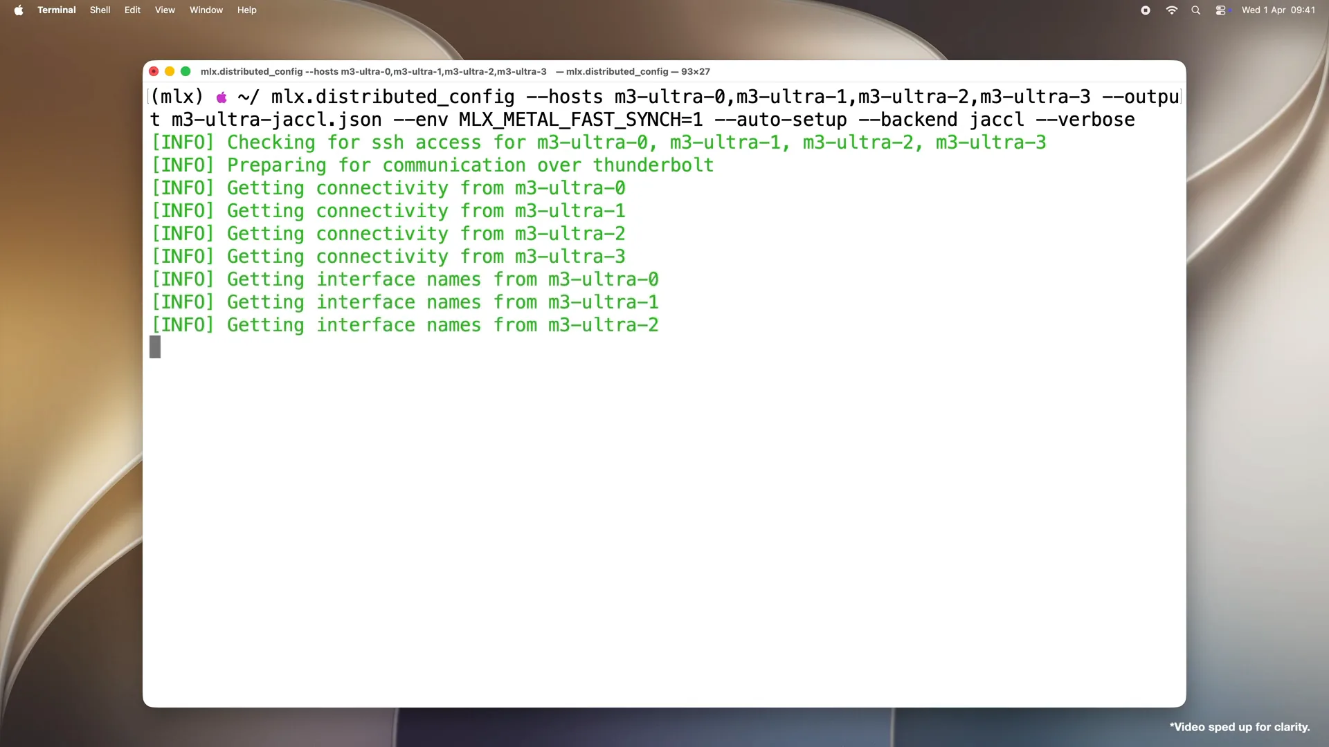 | First, it checks that all hosts are reachable over SSH. Then, it processes the connections by examining each machine's Thunderbolt ports to determine which machines are physically connected to each other, thereby building a map of the topology. |
Slide 40 — 10:22 (watch)
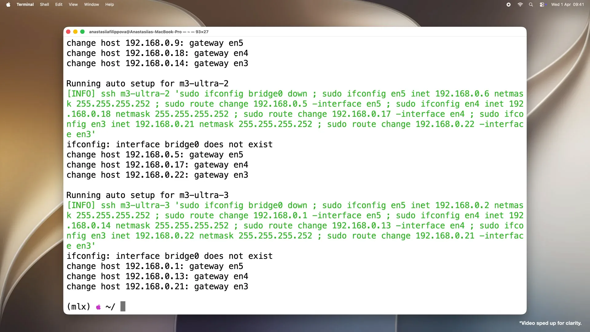 | Since we passed autosetup, the script disables the Thunderbolt bridge on all machines and configures each Thunderbolt link for RDMA. Finally, it writes a JSON host file containing everything needed for the MLX launch. Note that without the autosetup flag, the script prints the configuration commands for your review, allowing you to run them manually. |
Slide 41 — 10:38 (watch)
 | The cluster is now ready. We will move on to the exciting part: distributed language model inference and fine-tuning. The easiest way to begin this is through the command-line interface and MLX LLM. |
Slide 42 — 10:58 (watch)
 | MLX LLM is an open-source Python package built on MLX that provides command-line tools and a Python API for running language models locally on Apple Silicon. To get started on a single device, check out our video, "Explore Large Language Models on Apple Silicon with MLX" from WWDC25. |
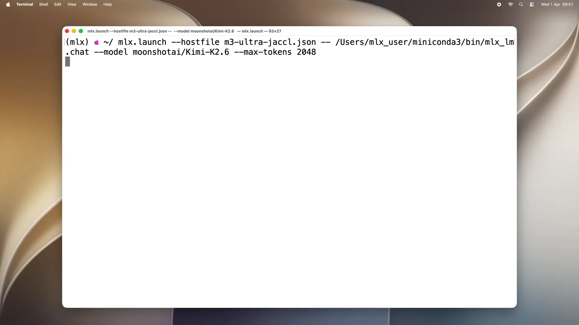
Slide 43 — 11:40 (watch)
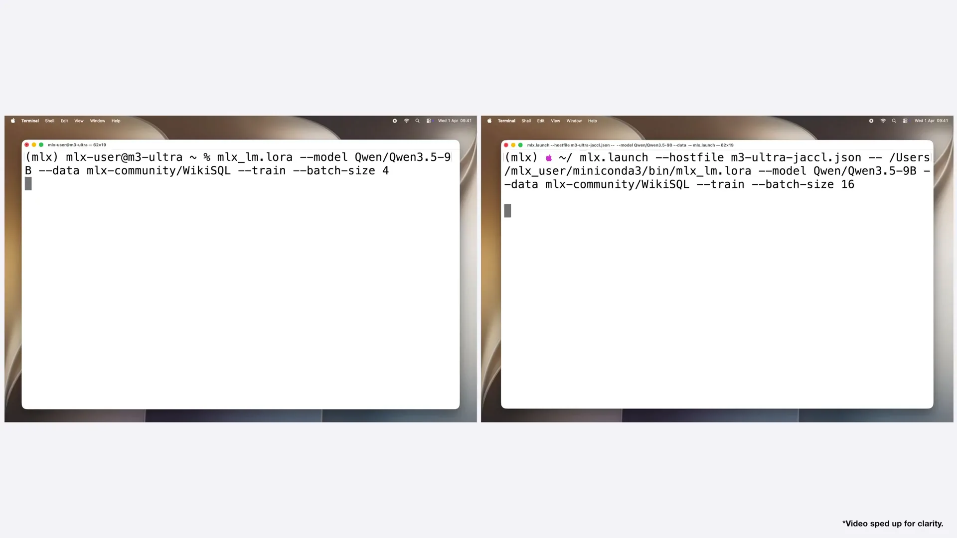
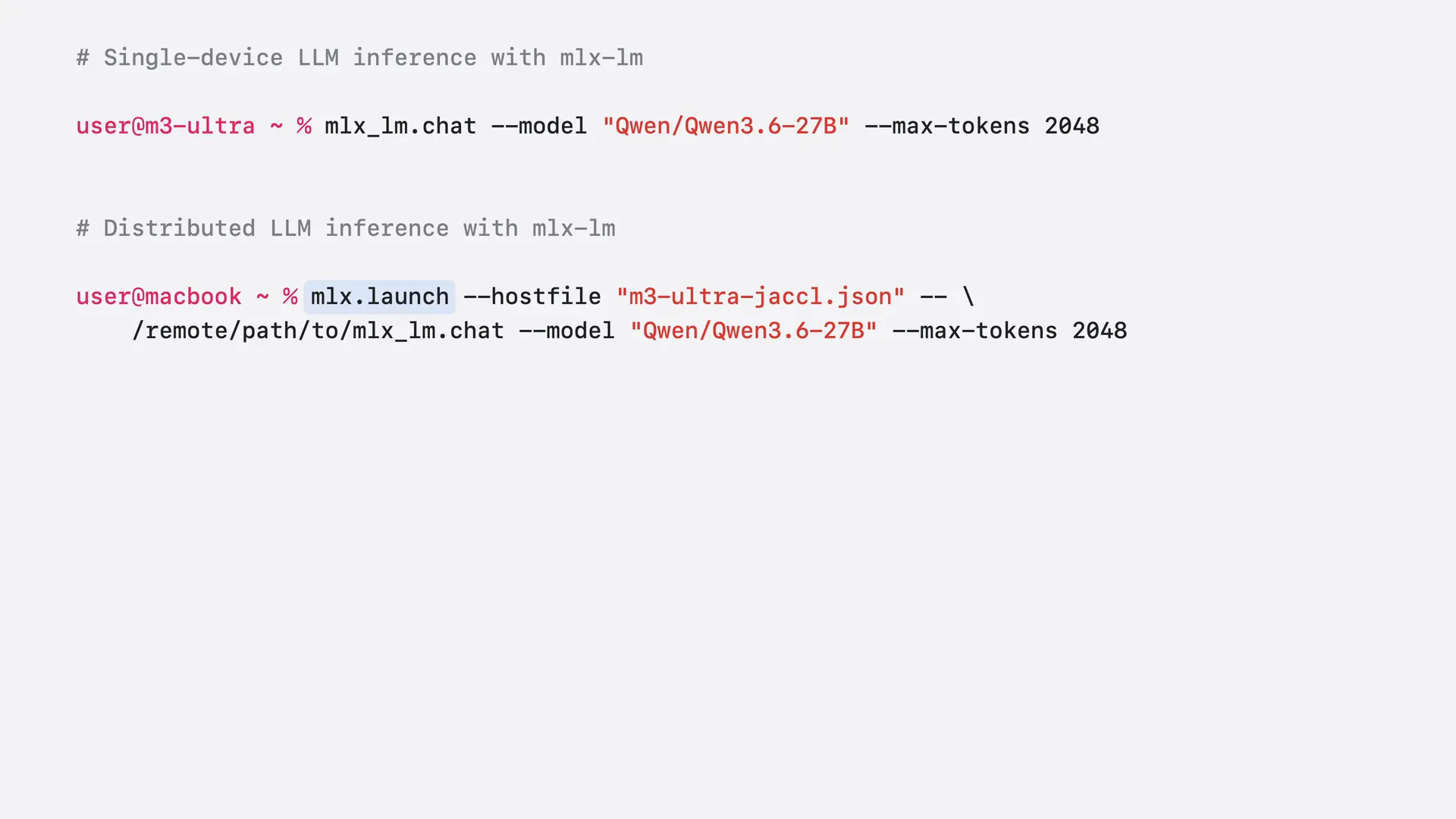 | As we demonstrated last year, you can chat with a model on a single Mac using the command-line interface with MLX LLM chat. You run it in the terminal, specifying the model, such as QN3.6, and the maximum number of tokens for the response. MLX LLM loads and runs the model on a single machine. To chat with the same model on the cluster via the command-line interface, you wrap the command with MLX launch. On your MacBook, you run MLX launch in the terminal with the host file pointing to your cluster configuration. After the double dash, you pass the same MLX LLM chat command, but with the remote path to the executable on each node. The command is nearly identical. MLX LLM manages the model and coordinates the distributed inference for you. Remember that all necessary libraries, including MLX, must be installed on each Mac, and the executable must be accessible on all machines. |
Slide 44 — 12:22 (watch)
 | With a single command in the command-line interface, we can run a model distributed across the entire cluster. We will compare the performance of QN3.6, a 27 billion parameter model, running on a single M3 Ultra versus four M3 Ultra machines. |
Slide 45 — 12:42 (watch)
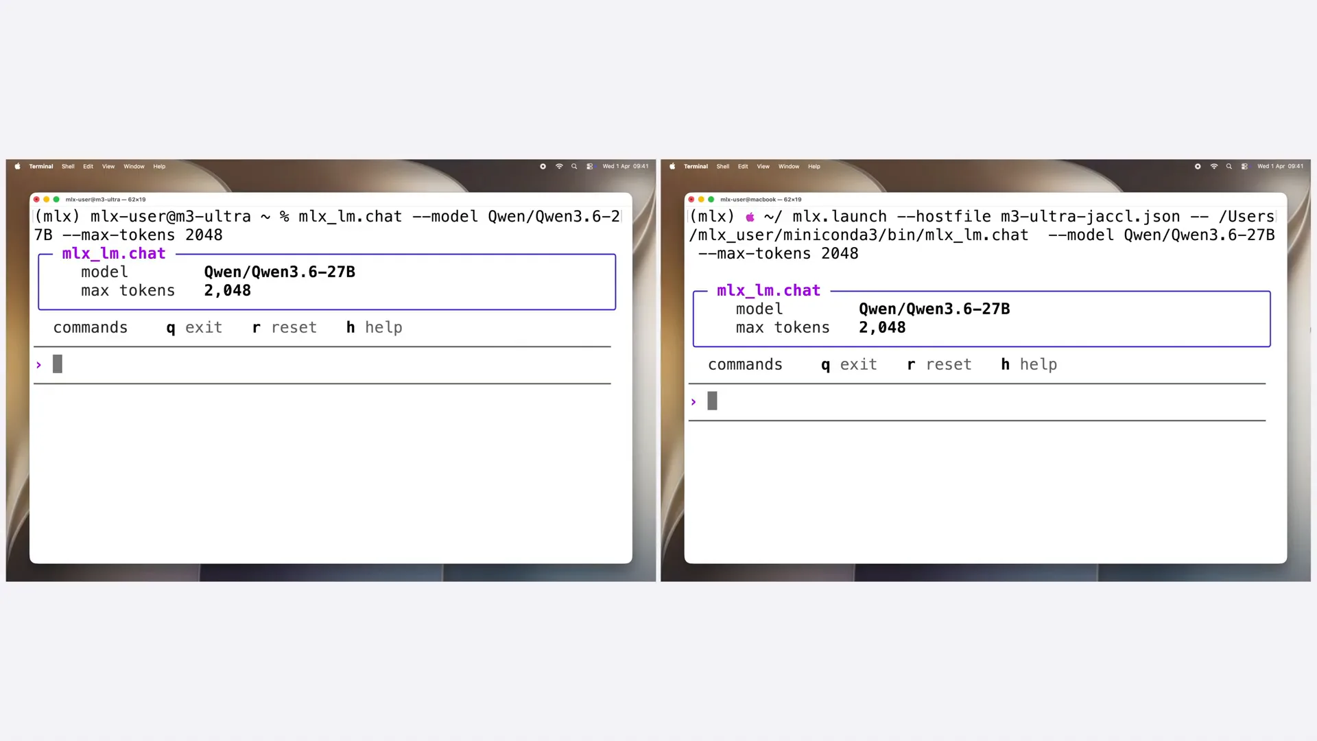 | I have already started the MLX LLM chat on both sides. On the left, the model is loaded on a single M3 Ultra, while on the right, it is sharded across four machines. Let's prompt both to implement a transformer model in MLX. |
Slide 46 — 12:54 (watch)
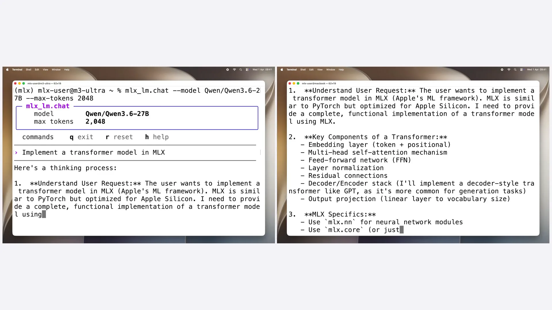 | The cluster generates tokens at nearly three times the rate of a single machine for the QN3.6 model, which is quite an impressive speedup. |
Slide 47 — 13:22 (watch)
 | Running a model across multiple Macs can significantly boost inference speed. The exact speedup depends on the model size and architecture. However, time improvement is not the only reason to adopt a distributed approach. Sometimes, a model is simply too large for one machine. For example, Kime 2.6 has one trillion total parameters. Even with 8-bit quantization, the weights alone require about one terabyte of memory. This amount does not fit on a single M3 Ultra but could fit across four machines. To split the weights and computation across machines, MLX and MLX LLM support two approaches: pipeline and tensor parallelism. |
Slide 48 — 13:58 (watch)
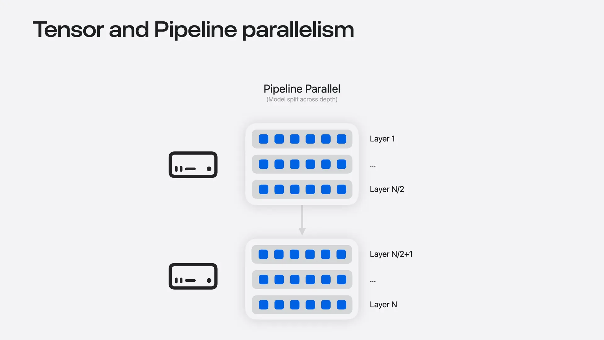 | Pipeline parallelism divides the model by depth, with each machine holding a group of layers. Data moves through the machines sequentially. While this approach does not accelerate inference—since each token must pass through the layer groups one after another—it simplifies communication. Machines only exchange activations at the boundaries between layer groups. |
Slide 49 — 14:24 (watch)
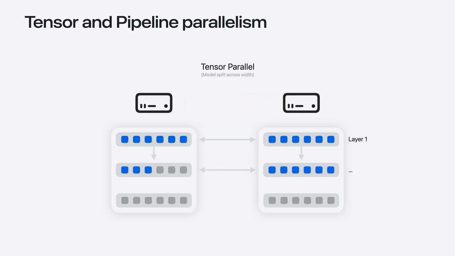 | Tensor parallelism splits the model by width, allowing each machine to hold part of every layer. This enables all machines to process the same token simultaneously, improving inference speed through parallelized per-layer computation. However, this approach requires much more frequent communication, occurring at every layer and for every token. |
Slide 50 — 14:42 (watch)
 | Low latency is important, which is why the mesh topology is crucial in this scenario. Every machine can reach every other machine in a single hop. |
Slide 51 — 14:54 (watch)
 | Tensor parallelism is the default sharding strategy in MLX for LLMs. To shard the model using pipeline parallelism, append the flag "pipeline" to the command. However, not all models support pipeline parallelism. |
Slide 52 — 15:06 (watch)
 | Now, let's shard a one trillion parameter Kimi2.6 on our cluster. |
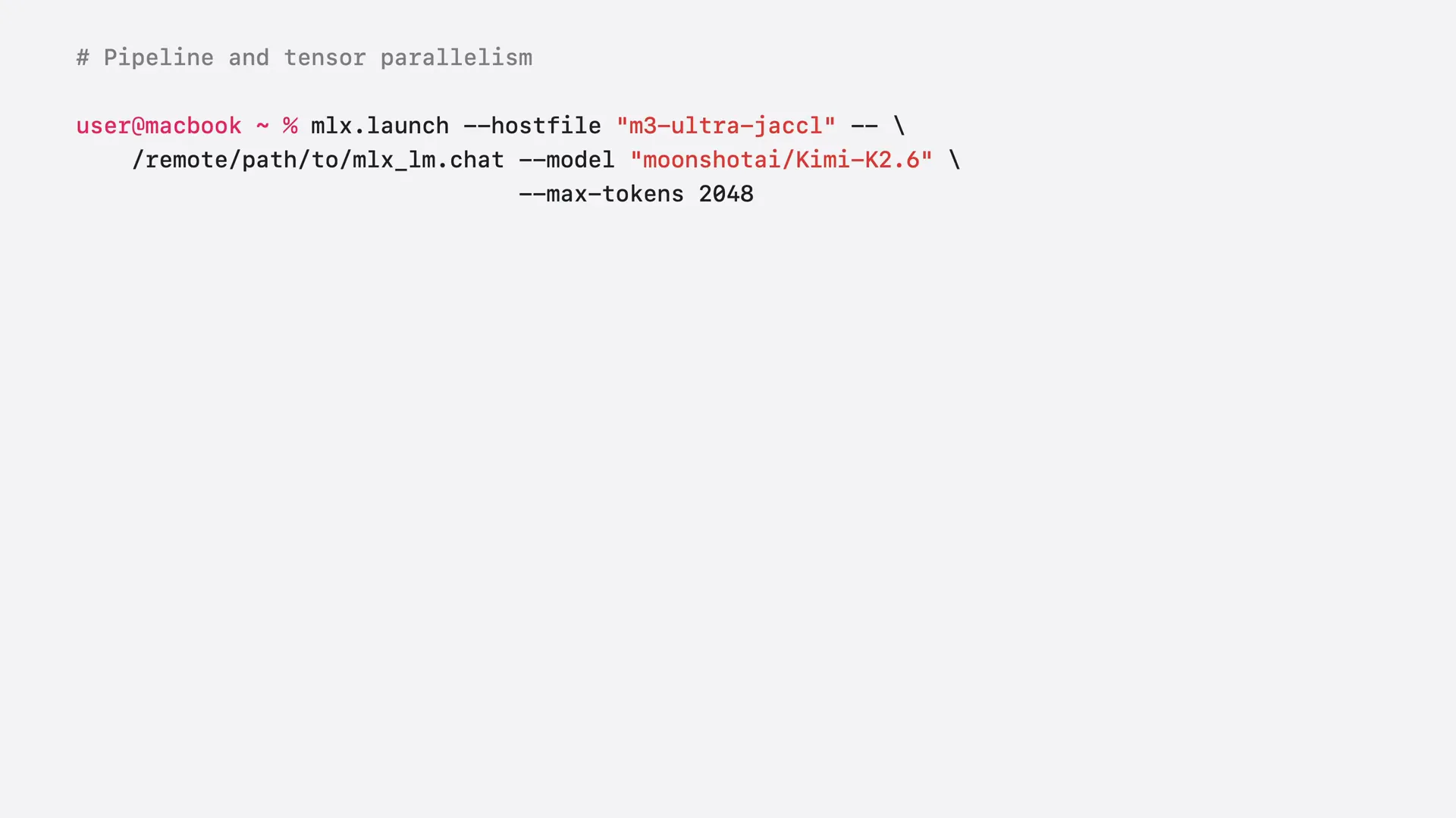
Slide 53 — 15:20 (watch)
 | For this, we use MLX launch from our MacBook as before, pointing to the host file. I am not passing the pipeline flag, so we are using tensor parallelism. We need to wait a moment while MLX launch connects to every machine. MLX LLM loads and shards the model, then starts the job. |
Slide 54 — 15:36 (watch)
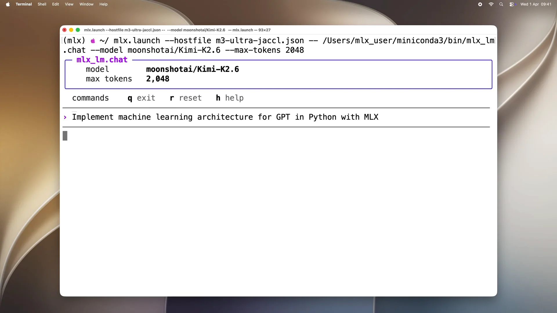 | The model is loaded. Let's prompt the model with "implement machine learning architecture for GPT in Python with MLX." With one command, a massive trillion-parameter model is running locally across your machines, answering your questions. |
Slide 55 — 16:02 (watch)
 | With MLX and MLX LLM, you can run language model inference and fine-tune models on your hardware. This process is fast, efficient, and fully private, ensuring that your data never leaves your machines. We will start with a single machine and then scale to our cluster. |
Slide 56 — 16:22 (watch)
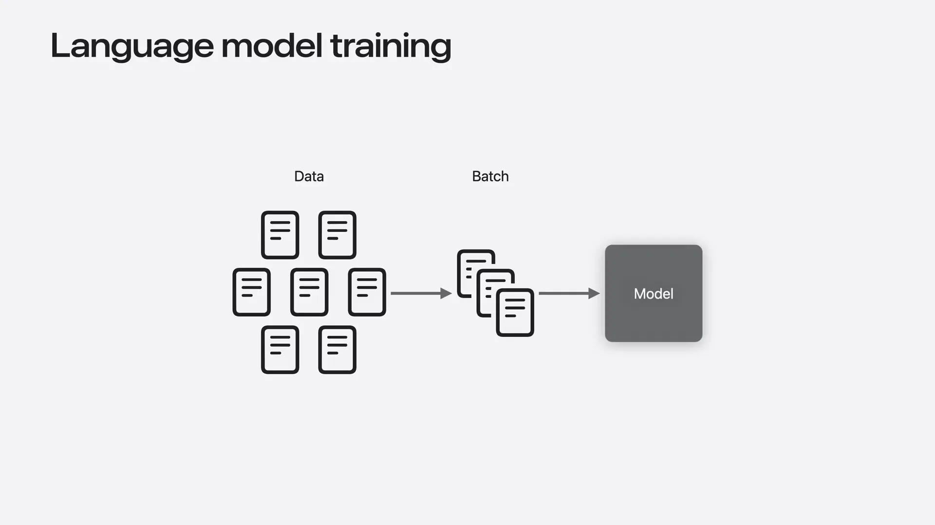 | When fine-tuning or training on a single machine, we split the training data into batches, which consist of multiple examples. For each batch, the mug computes gradients and updates the model weights. This process is repeated for one or more passes over the training dataset until the model achieves the desired quality. |
Slide 57 — 16:36 (watch)
 | The faster we process the training data, the sooner fine-tuning is completed. To achieve this, we can utilize multiple machines to accelerate the process. |
Slide 58 — 16:54 (watch)
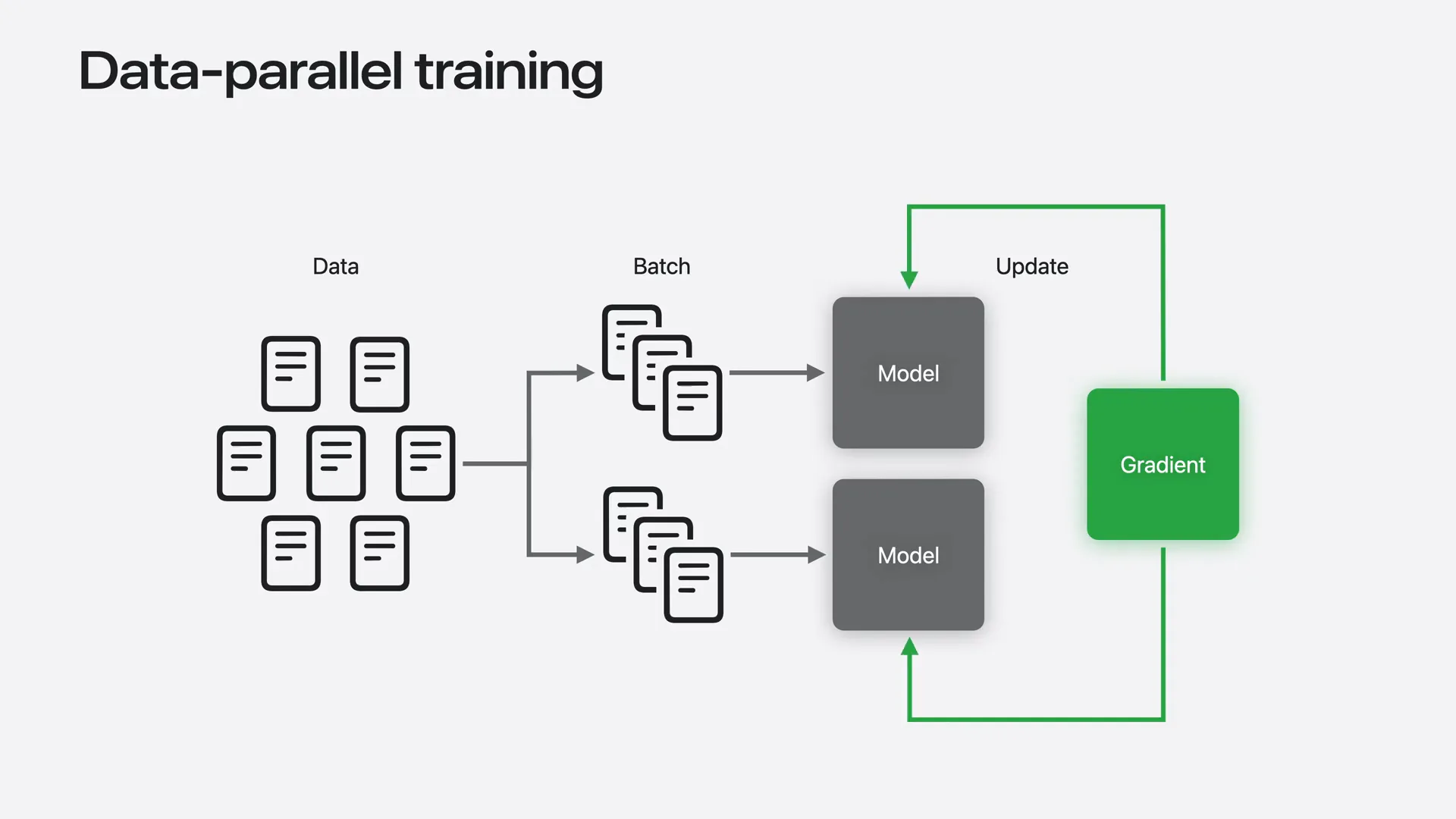 | The idea is straightforward. We replicate the model on every machine. Each machine receives a different batch of data and computes gradients locally. Then, we average the gradients so the model's update incorporates information from all batches. This approach is called data parallel training because the model is replicated while the data is processed in parallel across machines, resulting in a significant speedup. |
Slide 59 — 17:10 (watch)
 | With n machines, we can process data up to n times faster. This is a significant advantage. |
Slide 60 — 17:14 (watch)
 | We can utilize data parallelism with MLX LLM. |
Slide 61 — 17:30 (watch)
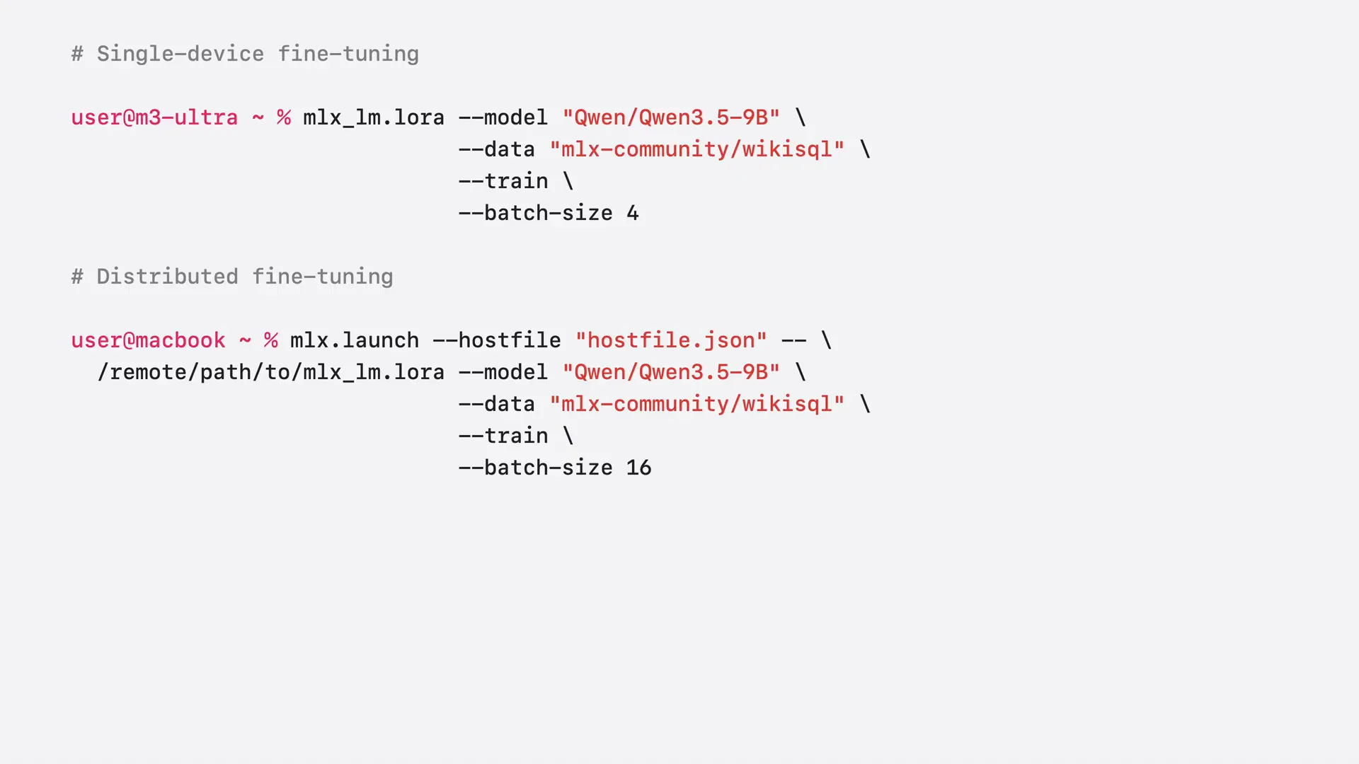 | The only difference from a single device is launching the job with MLX Launch from your MacBook and specifying a path to the MLX LLM LoRa on remote machines. Data sharding is managed by MLX LLM, and the command is nearly identical. We scale the batch size by the number of devices, ensuring that each machine processes the same number of samples per step as before. |
Slide 62 — 17:48 (watch)
 | We will fine-tune QN3.5, which has 9 billion parameters, on both a single machine and a cluster. We will compare the number of tokens processed by the model per second in each case. |
Slide 63 — 18:00 (watch)
 | We are launching fine-tuning on a single device on the left and on the cluster on the right using MLX. We utilize the launch and host file to specify the path to the MLX LLM LoRa on the remote machine. |
Slide 64 — 18:16 (watch)
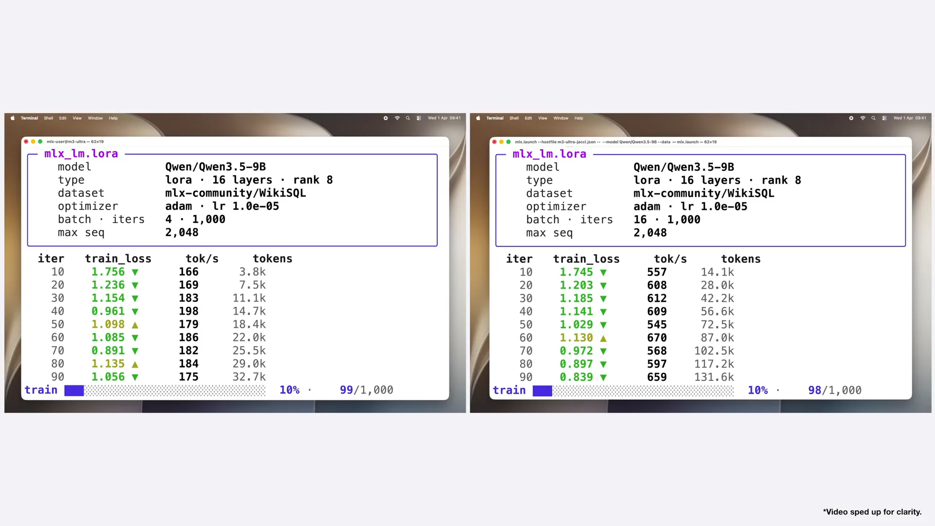 | First, it loads the data and model, and then training begins. A single M3 Ultra processes approximately 180 tokens per second, while the cluster processes around 600 tokens per second, resulting in more than a threefold speedup for fine-tuning. |
Slide 65 — 18:30 (watch)
 | With MLX, you can transform your devices into a local training cluster for efficient fine-tuning without relying on the cloud. |
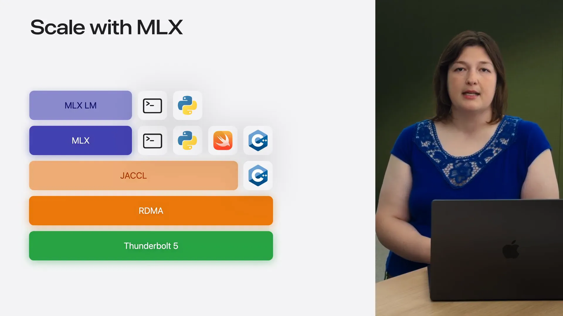
Slide 66 — 18:46 (watch)
 | So far, we have used the command-line interface for distributed inference and fine-tuning within the MLX LLM. However, MLX offers fine-grained control over sharding and distributed operations through flexible Python, Swift, and C++ APIs. This enables you to experiment with models in Python and C++ or embed models into your app using Swift. Let's look at the examples. |
Slide 67 — 19:14 (watch)
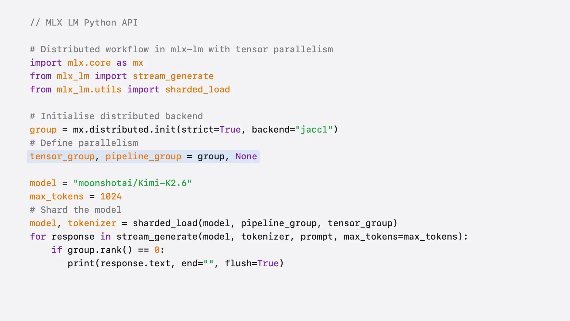 | To run distributed inference with the Python API and MLX LLM, we first initialize the distributed group for communication. Next, we define the type of parallelism we want, such as tensor parallelism. Then, we shard the model using the sharded load function. After that, we can use the model just as we would on a single device, as MLX LLM manages all distributed communications automatically. |
Slide 68 — 19:36 (watch)
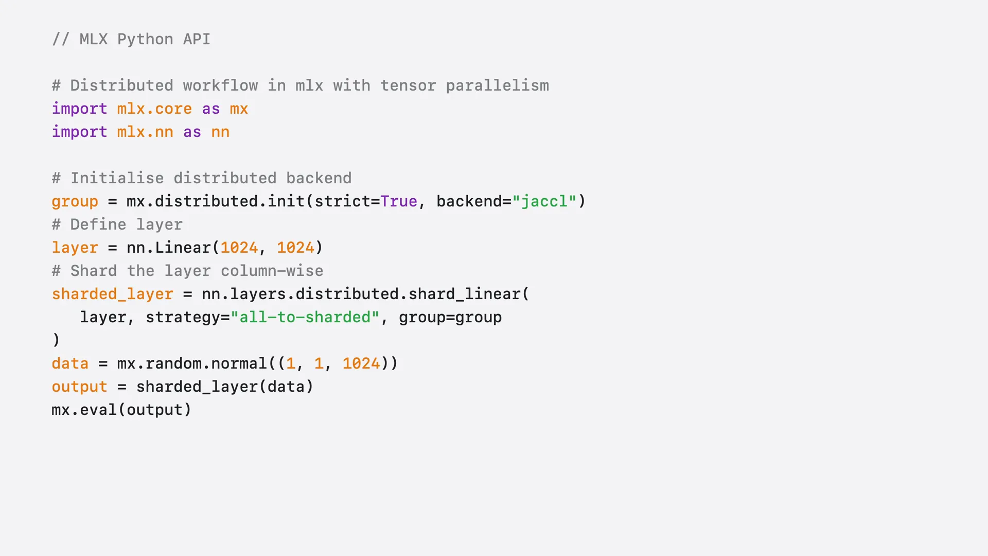 | To gain more control over the model and its sharding, we can use low-level primitives from MLX. For instance, after defining a simple linear layer, we can shard it with tensor parallelism using the shard linear function. |
Slide 69 — 19:52 (watch)
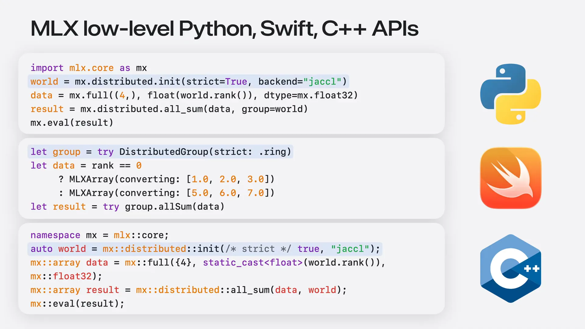 | You can control basic distributed operations, such as all-reduce, in Python, Swift, or C++. After initializing the distributed group using Jackal, we perform a collective distributed sum across all marks for our tensor with the corresponding MLX prism. |
Slide 70 — 20:16 (watch)
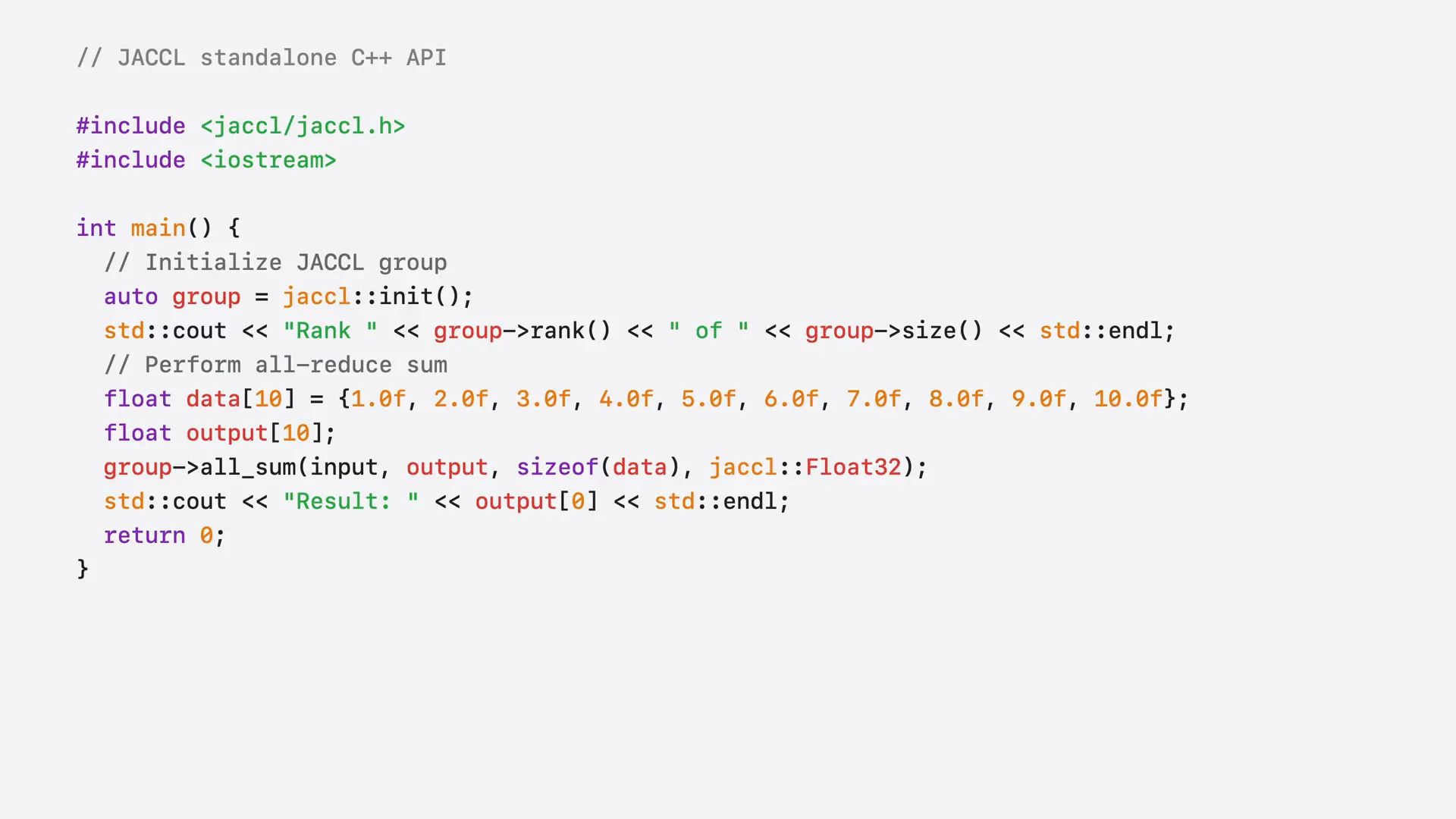 | As mentioned at the beginning of the session, Jackal is available independently and can be utilized for any applications that require distributed communication, including non-ML applications. Jackal can be built without MLX and offers a C++ API with communication primitives. After initializing a Jackal group, we perform a collective distributed sum across all marks for our tensor directly through Jackal, rather than using MLX. |
Slide 71 — 20:38 (watch)
 | You now understand both the high-level and low-level APIs for distributed inference and training with MLX and Jackal. You are prepared to build advanced distributed workloads using MLX. |
Slide 72 — 21:04 (watch)
 | Throughout the session, we explored the full stack that enables distributed training and inference on Apple Silicon, from RDMA over Thunderbolt to MLX and MLXLM. We demonstrated how easy it is to scale from a single device to multiple devices, highlighting the benefits such as faster inference, the capability to run trillion-parameter models, and quicker fine-tuning, all with minimal changes to your single-device code. This supports command-line interface, Python, Swift, and C++ APIs. |
Slide 73 — 21:26 (watch)
 | With Distributed Cluster, you can now run local AI agents powered entirely by MLX, quickly and privately, on your own hardware. |
Slide 74 — 21:42 (watch)
 | To learn more, watch our WWDC 2026 video, "Run Local Agentic AI on the Mac Using MLX." For advanced distributed features, including custom parallelism strategies and training loops, refer to our documentation. You can also use MLXLM to serve models in a distributed manner with the built-in server. |
Slide 75 — 21:56 (watch)
 | We look forward to seeing what you create with MLX on Apple Silicon. |